There is an has been an implementation for Little’s test for missingness completely at random (mcar) (Little 1988) in the R-package BaylorPsychEd. However, its implementation relies on the suggested R-package mvnmle (multivariate normal maximum-likelihood estimation), which stopped being available too (at the time of writing this post) and has been assigned the status of orphaned. For those, like me, who just like to run Little’s test on their data set, I fixed the deprecated dependency using the norm R-base package. You can download/ clone it from GitHub: rcst/little-test.
The differences to the orginial version from BaylorPsychEd in detail are:
- Replaced dependency mvnmle package with the norm package
- The function now ignores data rows where every variable is missing (which previously caused the function to crash)
Background
If you happen to statistically analyse a data set with missing values and you don’t want/ to can’t discard rows of data with missing values, then this post might be interesting for you.
Data sets can be incomplete in the sense that in a table-like structured data set of rows/ oberservations and columns/ variables, a certain fraction of the observations has missing values in some variables, usually denoted with NA as in not available. See for examble the following data set:
library(data.table)
library(knitr)
n <- 50
dt <- data.table(id = 1:n,
         x = round(rnorm(n), digits = 2L),
         y = round(rnorm(n), digits = 2L),
         z = sample(x = letters[1:3],
                size = n,
                replace = TRUE))

dt[sample(1:n, size = floor(n*0.3)), x := NA]
dt[sample(1:n, size = floor(n*0.3)), y := NA]


kable(head(dt, 7), caption="Example data set with 30% missing values in each variable")| id | x | y | z |
|---|---|---|---|
| 1 | NA | 2.44 | c |
| 2 | 0.06 | NA | b |
| 3 | NA | -1.27 | a |
| 4 | NA | -0.13 | b |
| 5 | 0.88 | 1.20 | c |
| 6 | 0.59 | NA | c |
| 7 | NA | -1.71 | a |
Little’s test basically compares the estimated means of each variable between the different missing patterns. These leads to either the decision to use simple random imputation or to model the missingness mechanism and use that model for imputation. The former is appropriate if one can be certain that the means are not different for different missingness patterns, i.e. a non-significant result of the Little’s test. For a more detailed explanation about the different types of missingness see Gelman and Hill (2006).
Little himself “… expect[s] the test to be sensitive to departures from the normality assumption, and even under normality the asymptotic null distribution seems unlikely to be reliable unless the sample size is large.” (Little 1988). See figure 1 for simulation results.
Below is the re-implementation of Little’s test and a test run for this apparently small sample and few variables.
mcar <- function(x){
    if(!require(norm)) {
        stop("You must have norm installed to use LittleMCAR")
    }

    # if(!require(data.table)) {
    #   stop("Please install the R-package data.table to use mcar")
    # }

    if(!(is.matrix(x) | is.data.frame(x))) {
        stop("Data should be a matrix or dataframe")
    }

    if (is.data.frame(x)){
        x <- data.matrix(x)
    }

    # delete rows of complete missingness
    foo <- function(x) return(any(!is.na(x)))
    dd <- apply(X = x, MARGIN = 1L, FUN = foo)
    dd <- which(!dd, arr.ind = TRUE)
    if(length(dd) > 0)
        x <- x[-dd,]

    # define variables
    n.var <- ncol(x) # number of variables
    n <- nrow(x)  #number of respondents
    var.names <- colnames(x)
    r <- 1 * is.na(x)

    nmis <- as.integer(apply(r, 2, sum))  #number of missing data for each variable REWRITE
    mdp <- (r %*% (2^((1:n.var - 1)))) + 1  #missing data patterns
    x.mp <- data.frame(cbind(x,mdp)) # add column indicating pattern
    colnames(x.mp) <- c(var.names,"MisPat") # set name of new column to MisPat
    n.mis.pat <- length(unique(x.mp$MisPat)) # number of missing data patterns
    p <- n.mis.pat-1 # number of Missing Data patterns minus 1 (complete data row)


    s <- prelim.norm(x)
    ll <- em.norm(s)
    fit <- getparam.norm(s = s, theta = ll)

    # gmean<-mlest(x)$muhat #ML estimate of grand mean (assumes Normal dist)
    gmean <- fit$mu
    # gcov<-mlest(x)$sigmahat #ML estimate of grand covariance (assumes Normal dist)
    gcov <- fit$sigma
    colnames(gcov) <- rownames(gcov) <- colnames(x)

    #recode MisPat variable to go from 1 through n.mis.pat
    x.mp$MisPat2 <- rep(NA,n)
    for (i in 1:n.mis.pat){
        x.mp$MisPat2[x.mp$MisPat == sort(unique(x.mp$MisPat), partial=(i))[i]]<- i
    }

    x.mp$MisPat<-x.mp$MisPat2
    x.mp<-x.mp[ , -which(names(x.mp) %in% "MisPat2")]

    #make list of datasets for each pattern of missing data
    datasets <- list()
    for (i in 1:n.mis.pat){
        datasets[[paste("DataSet",i,sep="")]]<-x.mp[which(x.mp$MisPat==i),1:n.var]
    }

    #degrees of freedom
    kj<-0
    for (i in 1:n.mis.pat){
        no.na<-as.matrix(1* !is.na(colSums(datasets[[i]])))
        kj<-kj+colSums(no.na)
    }

    df<-kj -n.var

    #Little's chi-square
    d2<-0
    cat("this could take a while")

    # this crashes at the missingness pattern where every column is missing
    # this for-loop can be handled faster with plyr-function
    for (i in 1:n.mis.pat){
        mean <- (colMeans(datasets[[i]])-gmean)
        mean <- mean[!is.na(mean)]
        keep <- 1* !is.na(colSums(datasets[[i]]))
        keep <- keep[which(keep[1:n.var]!=0)]
        cov <- gcov
        cov <- cov[which(rownames(cov) %in% names(keep)) , which(colnames(cov) %in% names(keep))]
        d2 <- as.numeric(d2+(sum(x.mp$MisPat==i)*(t(mean)%*%solve(cov)%*%mean)))
    }

    #p-value for chi-square
    p.value<-1-pchisq(d2,df)

    #descriptives of missing data
    amount.missing <- matrix(nmis, 1, length(nmis))
    percent.missing <- amount.missing/n
    amount.missing <- rbind(amount.missing,percent.missing)
    colnames(amount.missing) <- var.names
    rownames(amount.missing) <- c("Number Missing", "Percent Missing")

    list(chi.square = d2,
         df = df,
         p.value = p.value,
         missing.patterns = n.mis.pat,
         amount.missing = amount.missing,
         data = datasets)
}
r <- mcar(dt)## Lade nötiges Paket: norm## Iterations of EM:
## 1...2...3...4...5...6...7...8...9...10...11...12...13...14...
## this could take a whiler[["p.value"]]## [1] 0.3512089r[["missing.patterns"]]## [1] 4r[["amount.missing"]]## id x y z
## Number Missing 0 15.0 15.0 0
## Percent Missing 0 0.3 0.3 0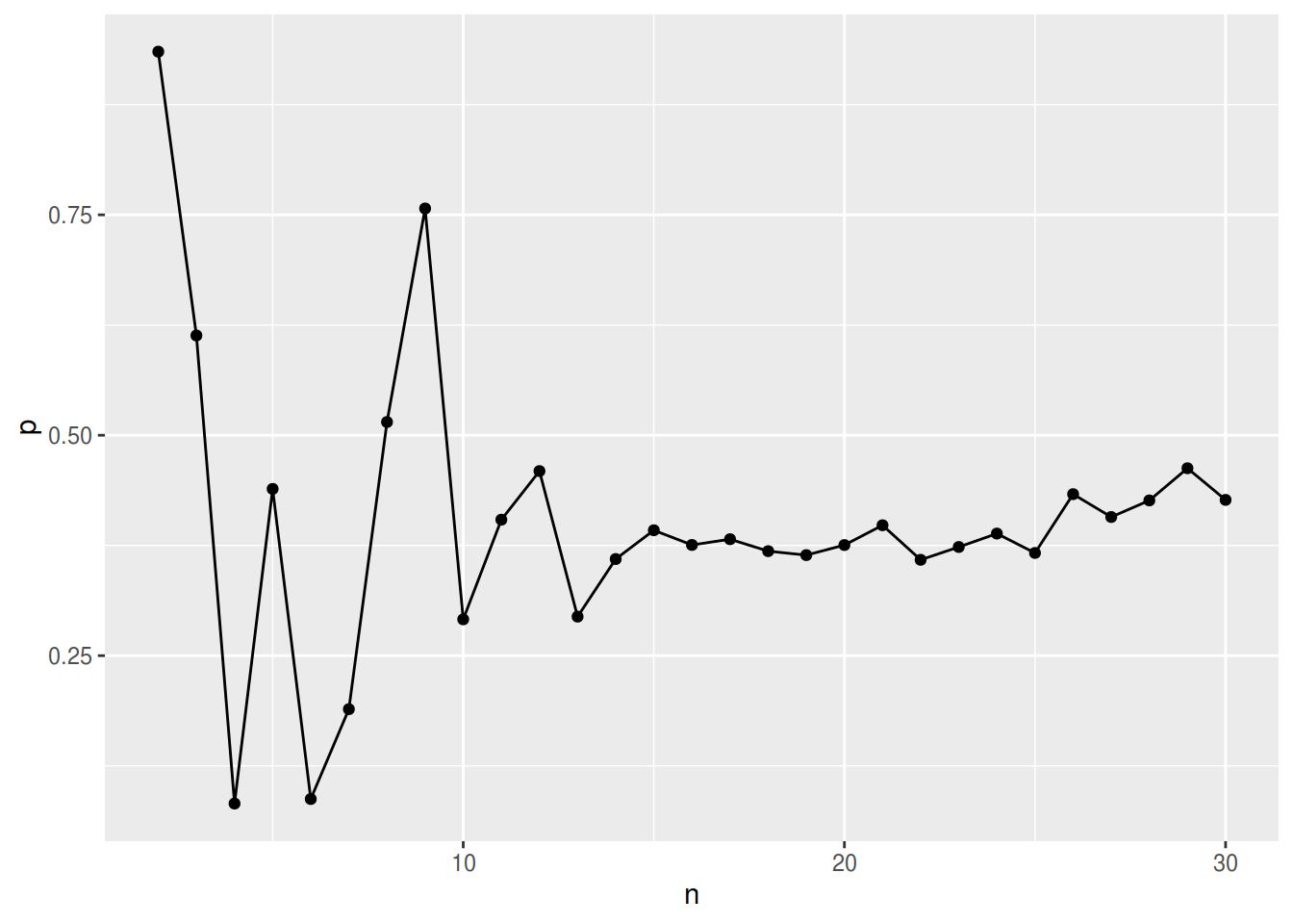
Figure 1: p-values for random data sets with different number of variables \(n\) at constant number of observations (100) with each 30% of missing data completely at random (mcar)
References
Gelman, Andrew, and Jennifer Hill. 2006. Data Analysis Using Regression and Multilevel/Hierarchical Models. Cambridge university press.
Little, Roderick JA. 1988. “A Test of Missing Completely at Random for Multivariate Data with Missing Values.” Journal of the American Statistical Association 83 (404): 1198–1202.
Comments