This is one of my posts of my self-study. It’s about estimating rat tumor rates from a number of experiments, where some treatment was applied to a number of of \(N\) rats and the outcome was the number of rats that grew a tumor. I’m posting here my solution of exercise 6.9 fom Gelman et al. (2013). This exercises itself is about model checking, but in order to do that one first needs to implement the Baysian model described in chapter 5.3.
I both enjoyed and cracked my head about this exercises, because it is quite rich in important aspects of Baysian modelling. One of the aspects covered in the model is reparameterization. Although it has been concisely described in the book. I will explain the reparameterization in my own words.
Reparameterization is here the trick to help find a hyperprior distribution, when a the standard uniform prior results in a improper posterior.
In this problem specifically we have a Binomial likelihood
\[ y_j \sim \text{Bin}\left(n_j, \theta_j\right) \]
for which a conjugate Beta prior population distribution is chosen for the \(\theta_j\)
\[ \theta_j \sim \text{Beta}\left(\alpha, \beta\right) \]
Now, as this is about hierachical modelling, we want a hyperprior distribution to estimate \(\alpha\) and \(\beta\) from the data as well. Instead of simply placing a uniform prior on both \(\alpha\) and \(\beta\), the first trick is to reparameterize in terms of mean and variance of the Beta distribution. In other words, we are converting our prior \(p\left(\alpha, \beta\right)\) into \(p\left(\frac{\alpha}{\alpha + \beta}, \frac{\alpha}{\beta}\right)\). In addition we can apply the log or also the logit() to both parameters, so that both parameters are defined in \(\left(-\infty, \infty\right)\).
This hyperprior has the advantage that we can easily interpret our estimates.
However, putting a uniform hyperprior distribution on those two parameters results in an improper posterior, i.e. it’s integral across the whole domain is not finite. At this point a hyperprior is proposed that basically is uniform on the mean and non-informative on the variance of the Beta (a standard choice for priors on variance parameters). The final result is then presented in the book, where it mentiones that “… which when multiplied by the appropriate Jacobian ….” As a newcomer to Baysian modelling, this sentenced left me puzzled, for which I didn’t understand the logic behind multiplying distributions by a Jacobian.
The full explanation is this: All probabilities of a variable must sum to one, or in the continuous case, must integrate to one. As long as a function has a finite integral, this can always be achieved by simply dividing the function by it’s “area under the curve” integral.
When we perform a parameter transformation of a function before integrating it, then the “area under the curve” changes by a factor which precisely is equal to the Jacobian. If that function is a probability distribution already, i.e. integrates to one we do not need to divide it anymore by it’s “area under the curve.” Hence, when we reparameterize a probability distribution, we simply need to multiply it by the Jacobian to maintain the “area under the curve.” For a more precise explanation on the interplay between integrals and Jacobians see it’s wikipedia page.
The rest of this post is my implementation of the model and finally the model checking. Based my model checks this model seems to be well fitting. If you have suggestions for a different test statistics, I would be happy to receive a comment.
Model checking for the rat tumor experiment
library(data.table)
library(plyr)
library(ggplot2)
library(patchwork)

dta <- data.table(n = c(20, 20, 20, 20, 20, 20, 20, 19, 19, 19, 19, 18, 18, 17, 20,
    20, 20, 20, 19, 19, 18, 18, 25, 24, 23, 20, 20, 20, 20, 20, 20, 10, 49, 19, 46,
    27, 17, 49, 47, 20, 20, 13, 48, 50, 20, 20, 20, 20, 20, 20, 20, 48, 19, 19, 19,
    22, 46, 49, 20, 20, 23, 19, 22, 20, 20, 20, 52, 47, 46, 24, 14), y = c(0, 0,
    0, 0, 0, 0, 0, 0, 0, 0, 0, 0, 0, 0, 1, 1, 1, 1, 1, 1, 1, 1, 2, 2, 2, 2, 2, 2,
    2, 2, 2, 1, 5, 2, 5, 3, 2, 7, 7, 3, 3, 2, 9, 10, 4, 4, 4, 4, 4, 4, 4, 10, 4,
    4, 4, 5, 1, 2, 5, 5, 6, 5, 6, 6, 6, 6, 16, 15, 15, 9, 4))


# grid for log(mean) and log(variance) of the hyperparameters
gdt <- CJ(pmean = seq(-2.3, -1.3, 0.01), psample = seq(1, 5, 0.01))
# gdt <- CJ(pmean = seq(-2.5, -1.0, 0.01), psample = seq(1.5, 3, 0.01))
gdt[, `:=`(alpha, exp(pmean) * exp(psample)/(exp(pmean) + 1))]
gdt[, `:=`(beta, exp(psample)/(exp(pmean) + 1))]

# log likelihood using the log-gamma due to computational overflow
gdt[, `:=`(part, sum(lgamma(alpha + beta) + lgamma(alpha + dta$y) + lgamma(beta +
    dta$n - dta$y) - lgamma(alpha) - lgamma(beta) - lgamma(alpha + beta + dta$n))),
    by = c("alpha", "beta")]
gdt[, `:=`(prior, alpha * beta * (alpha + beta)^(-2.5))]

# avoinding computational overflow: post -> log() -> substract max -> exp()
gdt[, `:=`(post, part + log(prior))]
gdt[, `:=`(post, post - max(post))]
gdt[, `:=`(post, exp(post))]

# needed for drawing random sample
gdt[, `:=`(post, post/sum(post))]
gdt[, `:=`(cp, cumsum(post))]


p1 <- ggplot(data = gdt, mapping = aes(x = pmean, y = psample, z = post)) + geom_contour() +
    xlim(-2.3, -1.3) + ylim(1, 5) + xlab("log(alpha / beta)") + ylab("log(alpha + beta)")
# draw random sample for alpha and beta on natural scale
N <- 1000
setkey(gdt, post)
gdt[, cp := cumsum(post)]
setkey(gdt, cp)
r <- data.table(ID = 1:N, rr = runif(N))
setkey(r, rr)
r <- gdt[r, roll = "nearest"]
p2 <- ggplot(data = r, mapping = aes(x = pmean, y = psample)) +
geom_point() +
xlim(-2.3, -1.3) +
ylim(1.0, 5.0) +
xlab("log(alpha / beta)") +
ylab("log(alpha + beta)")
p1 + p2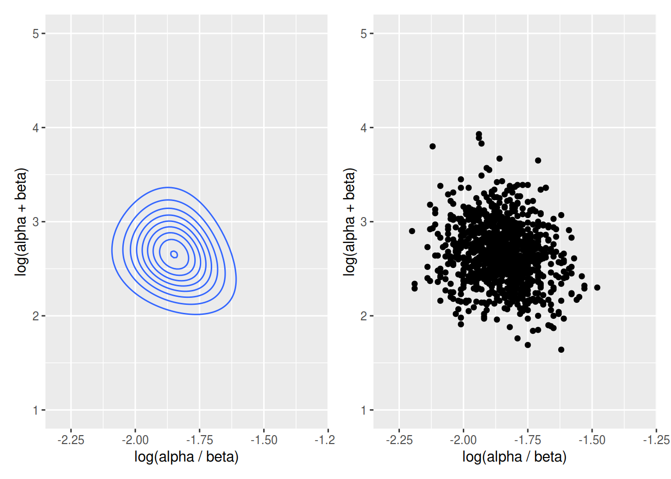
# for each draw of alpha and beta draw 71 thetas for each experiment
r[, paste0("theta", 1:nrow(dta)) := as.list(rbeta(n = nrow(dta),
                          shape1 = alpha,
                          shape2 = beta)),
by = c("alpha", "beta")]
mr <- melt.data.table(data = r, id.vars = 1:9)
p0 <- ggplot(data = dta, mapping = aes(x = y / n)) +
geom_histogram(binwidth = 0.01) +
theme_void() +
theme(plot.background = element_rect(colour = "black", size = 1))
# randomly select 10 replications
rid <- floor(runif(16, min = 1, max = 1000))
pl <- ggplot(data = mr[ID == rid[1]], mapping = aes(x = value)) +
geom_histogram(binwidth = 0.01) +
theme_void() +
theme(plot.background = element_rect(colour = "black", size = 0.5))
# plot in a grid side by side with the data
for(i in rid[-1]) {
p <- ggplot(data = mr[ID == i], mapping = aes(x = value)) +
geom_histogram(binwidth = 0.01) +
theme_void() +
theme(plot.background = element_rect(colour = "black", size = 0.5))
pl <- pl + p
}
p0 + (pl) 
dta[, p := y / n]
dta[, mean(p)]
## [1] 0.1321789gdt[, exp(sum(post * pmean))]## [1] 0.1576009ggplot(data = r, mapping = aes(x = theta1)) +
geom_histogram() +
geom_vline(xintercept = dta[, mean(p)]) +
annotate("text",
x = 0.25,
y = 90.0,
label = paste0("p = ", r[, sum(theta1 > dta[, mean(p)]) / .N]))## `stat_bin()` using `bins = 30`. Pick better value with `binwidth`.
Gelman, Andrew, John B Carlin, Hal S Stern, David B Dunson, Aki Vehtari, and Donald B Rubin. 2013. Bayesian Data Analysis. CRC press.
Comments