Background

I started teaching an introductory statistics course at the University of Khovd in January this year. For this reason I came across the book Teaching statistics: A Bag of Tricks (Gelman and Nolan 2017) which contains a number of in-class demonstrations to teach statistical concepts, from which I used “Real vs. fake coin flips” on day one in my class.

It pinpoints a common misconception about randomness, that I believe even trained scientist can fall victim to: patterns can occure randomly.

Fake vs. real coin flips

As described in the book, I divded my class into two groups where each group is supposed to generate the outcome of 100 coin flips. The first group takes an actual coin (or 10 coins for saving time) and flips it 100 times (or 10 times each coin) and writes down the result. The other group needs to come up with a sequence of coin flip results by generating a randomly looking sequence of coin flips. The results of this are two sequences of 0’s and 1’s.

In addition there is a blind judge who leaves the room while the flipping and writing happens and comes back to face the two sequences written on a blackboard. The judge is then asked to identify the real coin flips, in which he surprisingly succeeds. Theoretically.

In my case, I was also playing the judge and I didn’t know which sequence was real. I was utterly surprised when, (a) I myself was wrong in my educated guess, and the other judge was right and (b) I found out that the real-coin-flippers had not written down the sequence in the order in which they occured.

My first thought was that OK, that’s just bad luck and the fake-coin flippers did an actually good job at faking. But I realized that, as predicted by the book, the fake coin flippers did had very few runs on consecutive 0’s or 1’s. So I was wondering: Does shuffeling of a sequence independent trials change the distribution?

Let’s try it out!

Simulation

Here is a sequence of truely randomly generated coinflips:

set.seed(20210120)
a <- rbinom(n = 100, size = 1, prob = 0.5)
a

##   [1] 0 1 0 0 1 0 0 0 0 1 1 0 0 0 1 1 1 0 0 1 1 0 1 0 0 1 0 0 1 0 0 0 1 1 1 0 1
##  [38] 1 1 0 0 1 0 0 1 0 0 0 0 0 0 0 1 0 1 1 0 1 1 0 0 1 0 1 0 0 0 0 1 1 0 0 0 0
##  [75] 1 0 1 0 1 0 0 0 1 1 0 0 1 0 0 0 1 0 0 0 1 0 1 0 0 0

As mentioned above, patterns such as runs of 0’s or 1’s can occure and in this case are rather likely. The example above exhibits 53 runs from which the longest is of size 7.

Let’s see what happens, if we shuffle this sequence

as <- sample(a)
as

##   [1] 1 0 1 0 0 0 0 1 0 0 1 0 1 0 0 0 0 1 0 0 0 0 1 1 1 1 1 1 0 0 0 1 1 0 1 0 1
##  [38] 0 1 1 0 0 0 0 0 0 0 1 0 1 0 1 0 0 0 1 0 0 0 0 0 0 1 0 0 1 0 1 0 1 0 1 1 1
##  [75] 0 0 0 0 0 0 0 0 0 0 0 1 0 1 1 1 1 0 0 0 1 1 1 0 0 1

The resulting sequence has 47 runs of which the longest is of size 11.

But that’s just a single example. Let’s have a look on how shuffling affects random sequences in 1000 replications:

library(data.table)
library(plyr)
library(ggplot2)

dt <- data.table(ID = 1:1000)

foo <- function(x) {
    x <- as.data.table(x)

    a <- rbinom(n = 100, size = 1, prob = 0.5)
    as <- sample(a)

    x[, runs := length(rle(a)$length)]
    x[, longest := max(rle(a)$length)]

    x[, runs_shuffled := length(rle(as)$length)]
    x[, longest_shuffled := max(rle(as)$length)]

    return(x)
}

dt <- as.data.table(ddply(.data = dt, .variables = "ID", .fun = foo))

ggplot(data = dt, mapping = aes(x = runs, y = runs_shuffled)) +
    geom_point(position = "jitter") +
    geom_abline()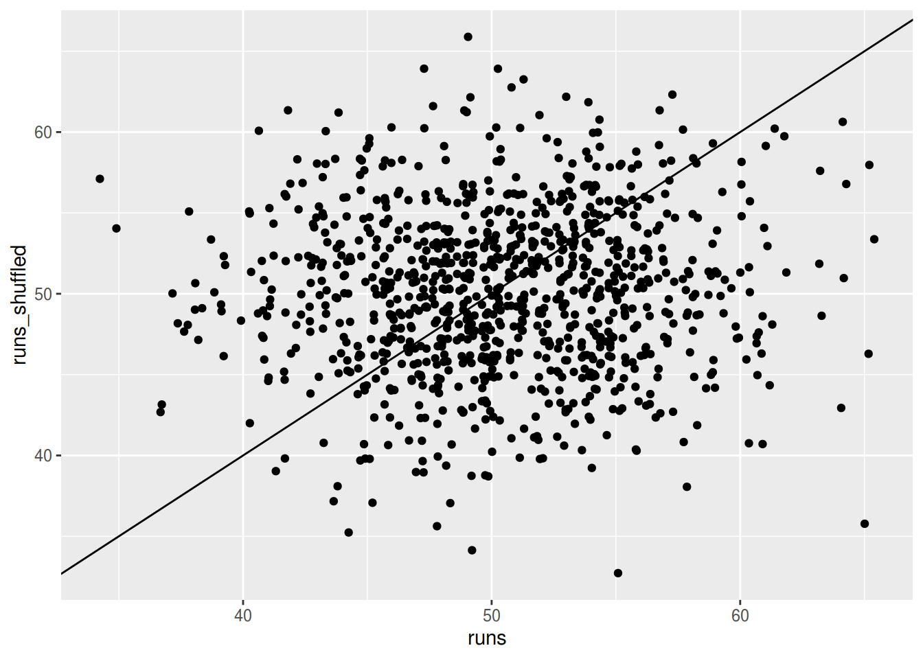

This plot tells us that shuffling on average does not affect the number of runs, since there are roughly as many points above the line as there are below (above: 46%, below: 47.5%). Due to the discreteness of the outcome, there are also cases in which the the shuffling didn’t affect the number of runs (6.5% in this case). However, when the original sequence’s number of runs is below or above it’s average, shuffling tends to “pull” it back towards average.

How about the maximum length of runs?

ggplot(data = dt, mapping = aes(x = longest, y = longest_shuffled)) +
    geom_point(position = "jitter") +
    geom_abline() +
    scale_x_continuous(limits = c(0, 17)) +
    scale_y_continuous(limits = c(0, 17))

## Warning: Removed 1 rows containing missing values (geom_point).

above: 42.3%, below: 39.3%

Conclusion

It seems like I simply had bad luck with this demonstration. Adding a layer of randomness by shuffleing does neither change the number of runs nor the longest observed run on average as it must, because the individual trials are independent. So the real coin flippers didn’t ruin their data by shuffling, in fact shuffling made it looking less extrem in case their un-shuffled data would have exhibited a less likely number of runs or length of longest run.