Annualization is when results that are with respect to a time period smaller then one year are scaled up so that it becomes with respect to one year. As a general principle this can also be called projection, grossing up, up-scaling, expansion or extrapolation.
In this article I want to implement and compare different methods for annualization (to stick with one term), in order to consolidate my own understanding of the topic. The method of choice is particularly easy to implement in R in a few lines of code and frames the problem of annualization in terms of missing data.
Example: Annual Ridership
One usecase for annualization can appear in survey analysis. The working example here will be from public transport: Imagine 3 riderhsip surveys are conducted in a city in 2023 to find out the total number of passengers travelling by bus per day. The ultimate goal is to estimate the annual ridership of this city. It is known that, due to seasonality, ridership varies throughout the year - e.g., it can be lower during summer. Hence the need to survey different periods of a year. Conducting surveys is an expensive and time-consuming endeavor, so that usually only a limited number of surveys can be conducted. In addition, another level of sampling comes into effect since usually it is impractical to survey every unit - in this case buses. Therefore, a number of certain buses are chosen among all the bus lines.
In total the procedure of analysing those surveys together can be summarized as in 2 steps:
For each survey, calculate an estimate of daily ridership that is representative for the period that the respective survey covers
Combine results and annualize to yield an annual total ridership
Data
We will create first a dataset to work with. For this, we will create three random periods of a year, each of length 4 weeks for which we will assume we have estimates of daily ridership - essentially having results ready from step number 1.
Corresponding to step number one, we will create what we can call a base data set which we will regard as a reference of true daily ridership. Simulating the conduncting of surveys this regard means that we get 3 averages of periods of 4 weeks.
Below is the code to create our base data. For the point of this article, we will also create a correlating factor for daily ridership, which in this case will be the number of performed kilometers, but more on will follow below.
library(data.table)
set.seed(20240528)
dt <- data.table(date = seq.Date(from = as.Date("2023-01-01"), to = as.Date("2023-12-31"),
    by = "day"))
dt[, kms := rnorm(n = 365, mean = 10 * (month(date) - 6)^2 + 500, sd = 25)]
dt[, ppd := rnorm(n = 365, mean = kms * 4, sd = 50)]
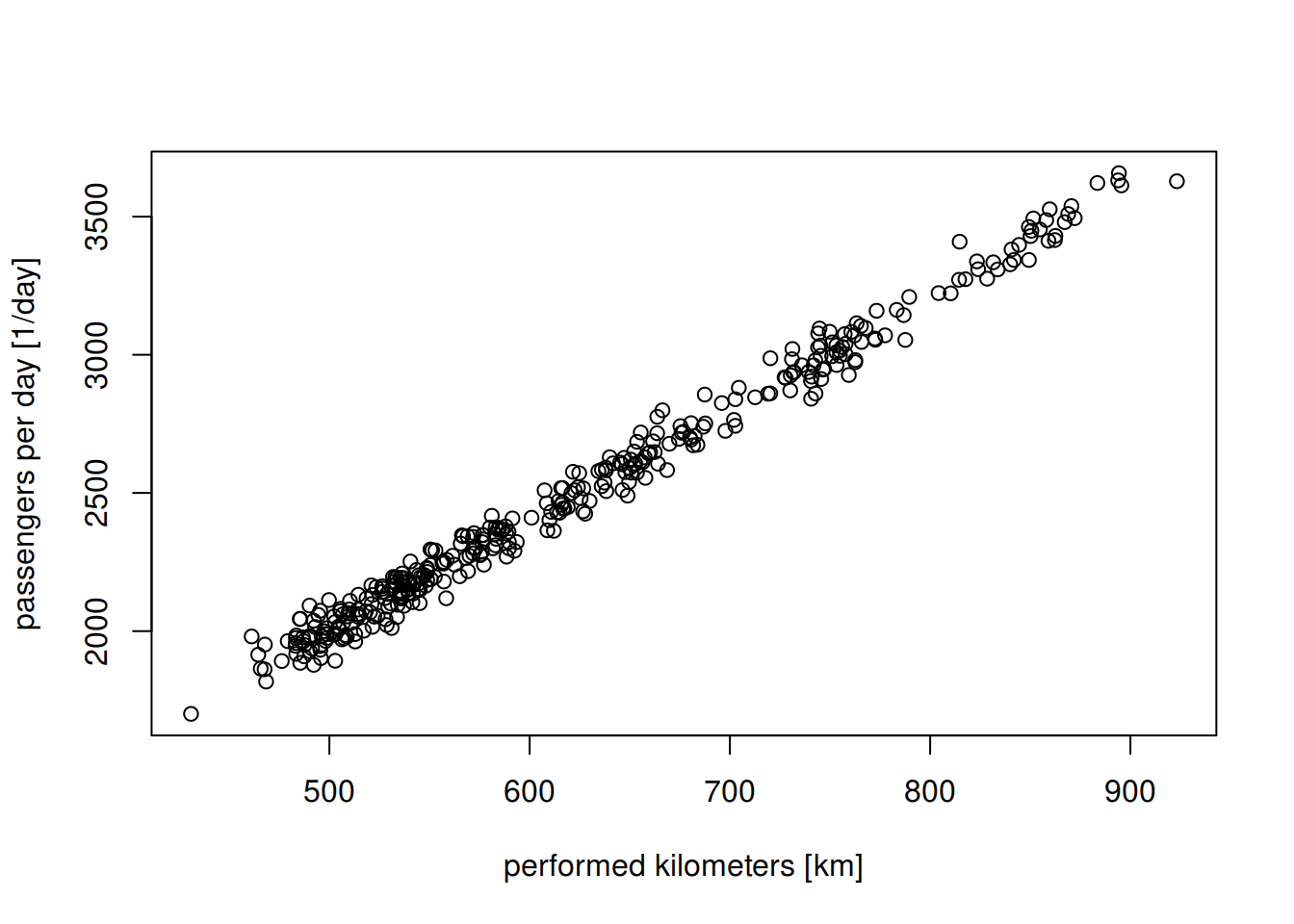
plot(dt$kms, dt$ppd, xlab = "performed kilometers [km]", ylab = "passengers per day [1/day]")
par(mfrow = c(1, 2))
plot(dt$date, dt$kms, xlab = "", ylab = "performed kilometers [km]")
abline(h = mean(dt$kms))
plot(dt$date, dt$ppd, xlab = "", ylab = "passengers per day")
abline(h = mean(dt$ppd))
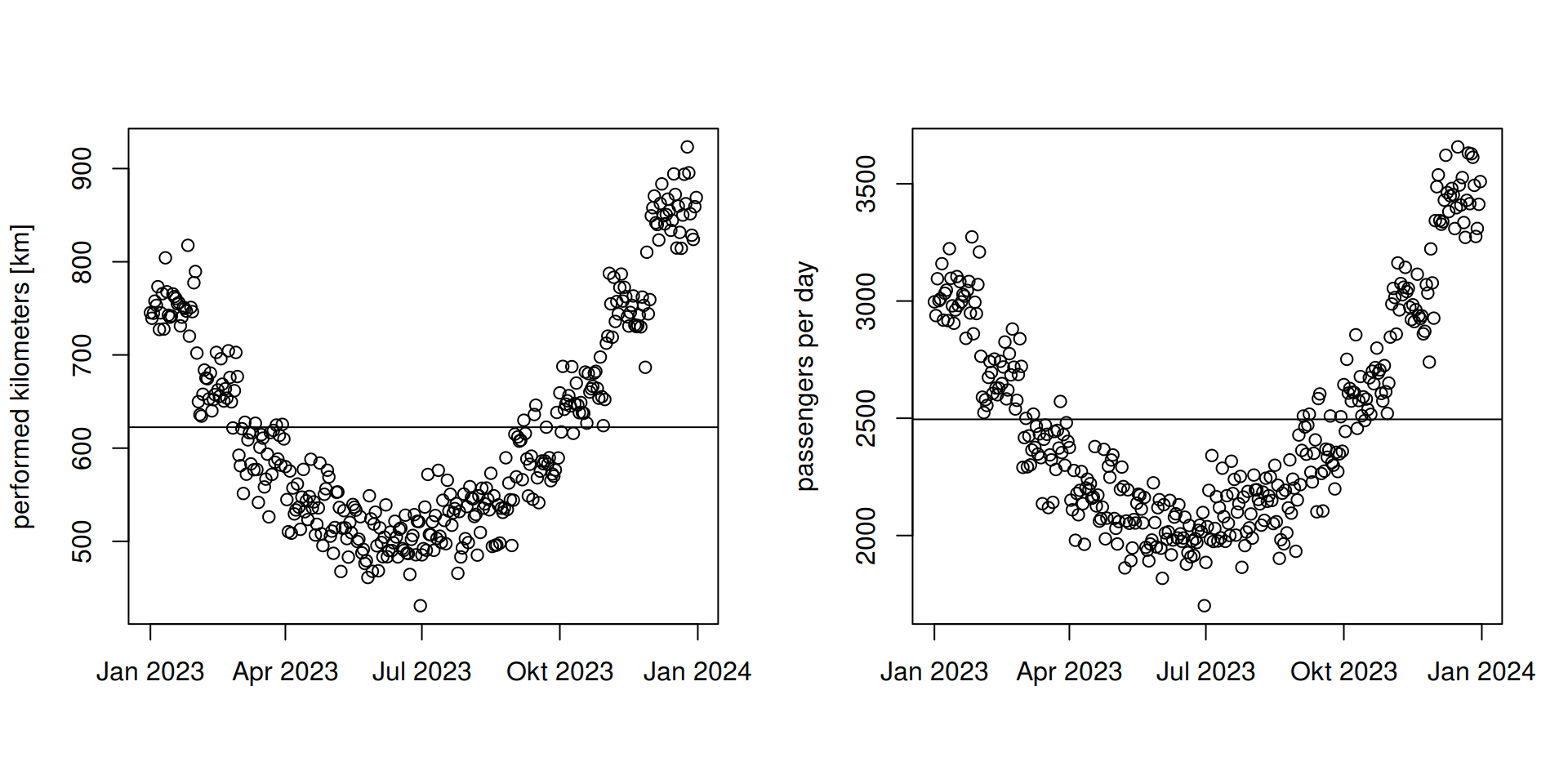
Figure 1: Seasonality of performed kilometers (left) and daily ridership (right). Horizontal line marks the average. Notice that the most representative months (closest to average) are April and October.
As we can see, we now have a dataset of daily ridership (ppd), which correlates with the number of performed kilometers (kms) and both are subsect to a seasonal trend (by month).
Now we will create survey results based on this - which effectively means observing only 3 periods of the dataset and averaging the observed ridership to a monthly mean. To simulate this, we will randomly create three periods. The tricky part is that we need those periods to be non-overlapping. For this, we’ll simply choose three different starting dates, test if they are at least 4 weeks (120 days) apart and if not try again.
In the next section we will calculate the annual ridership from those estimates and compare it to the true value.
repeat {
    # substract 31 days in December to ensure surveys are conducted within one
    # year we also want to make sure to get one survey in summer
    s <- sort(ceiling(c(runif(n = 1, min = 0, max = 179), runif(n = 1, min = 180,
        max = 180 + 2 * 31), runif(n = 1, min = (180 + 2 * 31) + 1, max = 365 - 31))))
    if (all(diff(s) > 40))
        break
}

# s <- as.Date('2023-01-01') + s
sdt <- data.table(survey_begin = as.Date("2023-01-01") + s)
sdt[, survey_end := survey_begin + (4 * 7)]
sdt <- dt[sdt, on = c("date>=survey_begin", "date<=survey_end")][, .(ppd = mean(ppd)),
    by = c(survey_begin = "date", survey_end = "date.1")]
print(sdt)
## survey_begin survey_end ppd
## <Date> <Date> <num>
## 1: 2023-01-07 2023-02-04 2966.356
## 2: 2023-08-22 2023-09-19 2279.425
## 3: 2023-10-10 2023-11-07 2705.054Method 1: Simple Mean
One way to annualize is to multiply a result by the number of instances it will occure in one year. In this case this could be 12, if we were to consider a result for a single month. If we had zero understanding of the generative process of the data, we could simply annualize all 3 surveys and take the average as combined result.
truth <- dt[, sum(ppd)]
error <- (sdt[, mean(ppd * 365)] - truth)/truth
The estimatation error is 6.2%.
Method 2: Weighted Mean
Method 1 underestimates the true number, since we are giving too much weight to summer periods that we know have a lower ridership. Probably a more informed way would be weight results according to our understanding of the estimates representativeness. Vaguely knowing that summer is different from the rest of the year, this could be expressed with two different weights for summer and off-summer. One way to choose weights is to use the inverse of the sampling probability. In this case this means the inverse of sampling a summer month vs. an off-summer month. In our case, we randomly chose three random 4 week periods. For simplicity, we will “round” the period to the more dominant month. The chance of picking a summer month (July or August) is \(\frac{2}{12}\) and to pick an off-summer month \(\frac{10}{12}\). So a summer month survey result will be weighted by a factor of \(\frac{12}{2} = 6\) and an off-summer survey results by \(\frac{12}{10} = 1.2\). This could also be justified by looking at the how much service level e.g., bus kilometers are performed during summer compared to off-summer for instance, and to realize that just because this it is much more likely to sample less buses in summer.
In R, we can use function weighted.mean for exactly this purpose.
sdt[, weight := mean(month(seq.Date(from = survey_begin, to = survey_end, by = "day"))),
    by = .(survey_begin, survey_end)]
sdt[, weight := fifelse(month(survey_begin) %in% c(7, 8), 12/2, 12/10)]
print(sdt)
## survey_begin survey_end ppd weight
## <Date> <Date> <num> <num>
## 1: 2023-01-07 2023-02-04 2966.356 1.2
## 2: 2023-08-22 2023-09-19 2279.425 6.0
## 3: 2023-10-10 2023-11-07 2705.054 1.2error <- (sdt[, weighted.mean(x = ppd, w = weight) * 365] - truth)/truthThe estimatation error is -2.29%.
Method 3: Linear Regression
Indeeed, method two improves the estimation error. Another way to look at the problem of annualization is to think of it as a dataset with missing data. In these terms, annualization is simply the sum of a value that is with respect to a single day. Having survey results for only parts of a year, another approach can be to estimate values for the missing days. In the context of missing data, if we where sure that the data is missing completely at ranom, we could simply re-sample data from the existing data as a replacement. However, in most cases (including this one), data is not missing completely randomly and it is usually better to use other known correlating factors. For this approach, the problem then is shifted to estimating surrogate values.
Missing value imputation can be done in R by using the package mice, which implementes so-called Fully Conditional Specification.
However, the basic idea of this is to use as much information as possible to estimate plausible imputations for missing data using regression.
As a demonstration, we will run a simple linear regression using our correlate of performed kilometers.
In order for this to work, we need to “expand” our survey data set to all days to get a dataset with missing entries in column ppd.
We can then run a simple base R regression using the lm() function, which by default will discard any rows for which there are missing entries in any of the outcome or predictor variables.
The resulting regression object can then be used in conjunction with base R’s predict() function to replace all missing occurrenences of ppd with our estimates.
# add kilometers performed during the observed survey periods
sdt <- sdt[dt, on = c("survey_begin<=date", "survey_end>=date")][, .(survey_begin,
    survey_end, weight, kms, ppd)]
reg <- lm(ppd ~ kms, data = sdt)
sdt[, ppd_est := predict(reg, newdata = sdt)]
error <- (sdt[, sum(ppd_est)] - truth)/truth
With this we get an estimatation error 1.23%.
Comments